

In the next of our blogs on Building a Digital Twin within the ArcGIS Platform, we look at extracting architectural detail and assets from the point cloud data of our offices we collected using a drone and a laser scanner.
Missed the early instalments of the series? Check out Part 1, Part 2, Part 3, Part 4, and Part 5 first.
Introduction
In the last blog we described how we created basic, but very usable, 3D models of our offices using the point clouds for reference. Our London office was quite well represented, but the architectural detail in our Leeds office features was largely lost – you can still appreciate the chimney breasts and high ceilings, though!
In this blog we look at a variety of (mainly experimental) techniques that we have developed to attempt to capture the finer details. Obviously we have the point cloud to refer to, but it has some limitations, and we’d ideally like to create models of specific features to which we can tie attributes.
We did trial a variety of other software packages in an attempt to find something suitable (such as CloudCompare – the link describes that product and gives a list of alternatives), but we didn’t find anything that we managed to get good (or in some cases, any) results from – this may, of course, say more about our limitations than the software’s! In any event, our initial aim was to do as much of the processing within the ArcGIS Platform as possible, so here’s what we did…
Select some targets
First we defined a few example targets to see how effectively we could capture them – bearing in mind that the primary reason for doing this was to define a baseline for the objects’ state, which could then be used for insurance and/or conservation purposes.
In the case of Listed Buildings, such as our Leeds office, this reasoning could be extended to argue that you could limit capture to the items explicitly noted in the Historic England listing entry– e.g. the deep moulded frieze with acanthus decoration below moulded ceiling cornice – which would at least put boundaries on the effort, and also provides some structure for this blog.

Figure 1 – Some acanthus with your deep moulded frieze?
So, we selected a few targets to look at, and we dealt with them in our initial perceived order of complexity:
- Cellar ceiling (not on listing, but a useful starting point)
- Library ceiling
- Exterior projecting carved portrait heads
Cellar ceiling
There are multiple rooms in the cellar. The two we will focus on both have brick-built vaulted ceilings.
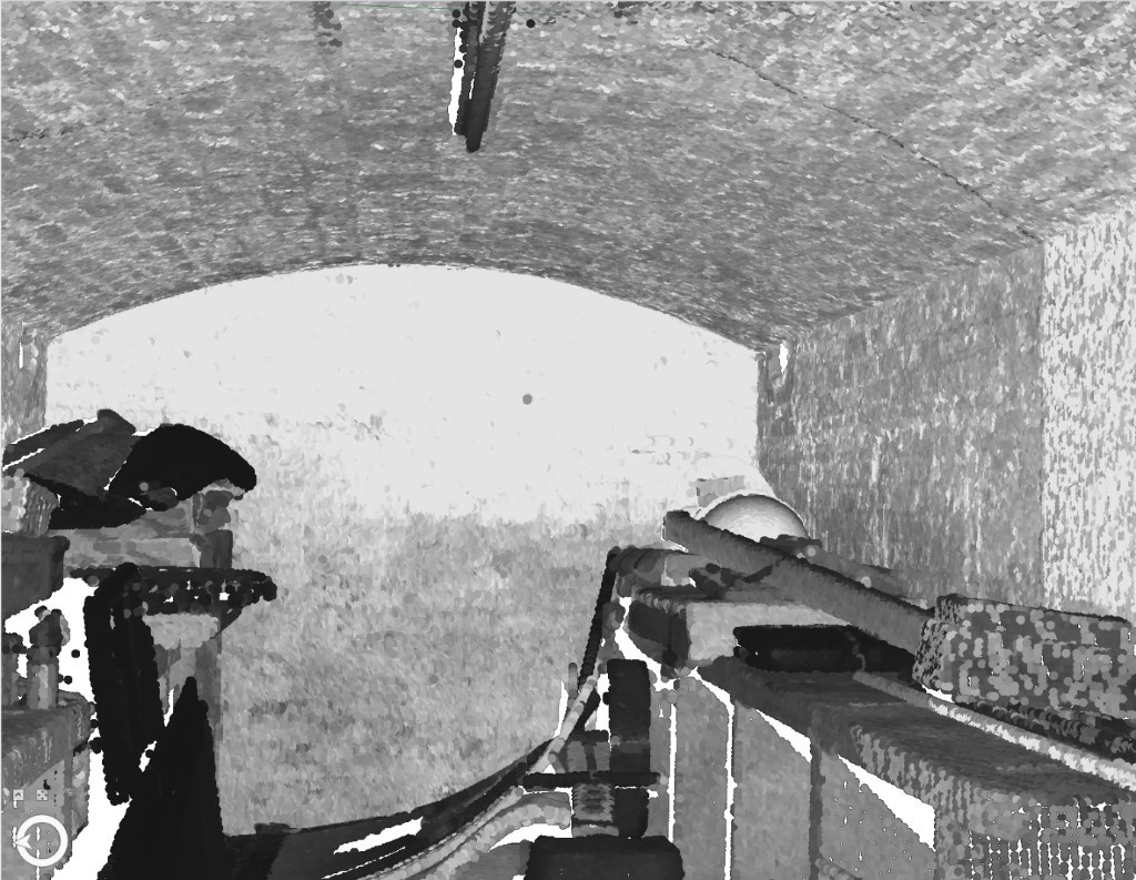
Figure 2 – Down in the cellars
Draw some lines
Having failed to find a built-in tool (spoiler: there is one) we scratched our heads and tried various things out – one that ought to have worked better involved digitizing intersecting 3D lines using the point cloud to snap the vertices to: the thinking being that we could then generate 3D polygons from the lines. Sadly, the execution of this was tedious and actually quite challenging, as the point to which it would snap would often be one behind the one you were aiming for, creating wonky lines. It also didn’t appeal as a convenient solution, so we moved on – but, as you’ll see, we came back to this concept later on.
If in doubt, grid it
As we have considerable experience using raster data sets, we thought we’d look at creating raster surfaces from the point clouds, which we could then convert to vectors or meshes. We had written some Python tools that allowed us to slice data out of point clouds, so we used these to extract the ceiling from the point cloud.

Figure 3 – looking up at the extracted ceiling point clouds in the cellar
We then created a tool that interpolated a surface at our desired resolution through the point cloud, and we used thinning based on the resolution to reduce the data volume. The result from running this tool at 1cm resolution is shown below, with an inset showing some detail. The ridge (or trough, depending on your perspective) is the fluorescent light, although of more interest perhaps are the individual bricks which are discernible towards the bottom of the inset.
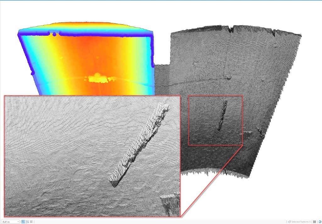
Figure 4 – The outlines of bricks
We were quite pleased with this result as it had accurately captured the shape of the ceiling and retained a considerable amount of fine detail. We improved the script to interpolate the colour and intensity information from the input point cloud, so that we could then style the polygons using these (using Arcade expressions – see below for further details).
There was a bit of an issue though – the output featureclass was large – as in we need a better graphics card large – I was doing this on my laptop, which has a 2Gb Nvidia Quadro M620; sadly the high-end graphics workstations were all out-of-bounds in the locked-down (and very well secured, he said quickly) offices. Nice though it was, it was clear this wasn’t going to fly as a mainstream approach – I.e. something that could generate content that could be used on a regular computer – but it would satisfy our specific requirement to capture a baseline.
Built-in tools
As we noted in passing above, there’s actually a 3D Analyst tool called LAS Building Multipatch which can be co-opted to do something similar to what we are trying to achieve. Using the extracted ceilings, we created a multipatch that has the correct ceiling curvature – the screenshot below shows the multipatch in green, offset for clarity from the point cloud, which is symbolized using elevation:
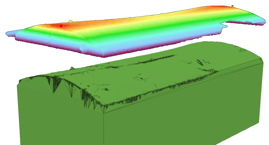
Figure 5 – a multipatch derived from a TIN derived from a point cloud
The result wasn’t bad – obviously there’s some noise around the edges, but, by specifying the wall height as an input parameter, we got the whole room as a single object, which is pretty impressive.
Library ceiling
Applying the LAS Building Multipatch tool to the library, we got an interesting result – again, we have a fully-formed room, and again we have noise around the edges – specifically the vertical planes. You wouldn’t want to give it to a builder and say ‘make that’, but it conveys the general form (see inset, view from above) quite well:
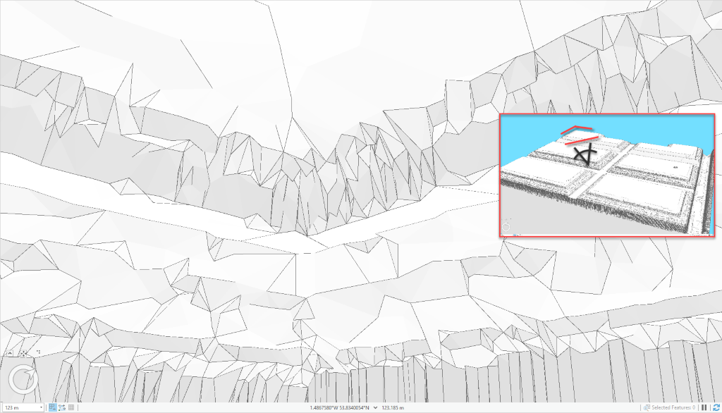
Figure 6 – Multipatch of the Library ceiling (see below for an improved view)
However, it doesn’t meet our ‘baseline’ requirement, so we repeated our home-grown approach – unsurprisingly, given it’s a bigger room, doing this at the same resolution generated an even more unwieldy (in fact, unusable on my laptop) dataset. We persisted, clipping out smaller areas to work with, and obtained a pretty good result at a resolution of 1mm, arguably meeting our requirement (especially if we increased the resolution):
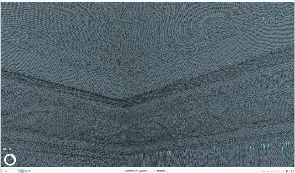
Figure 7 – A high resolution 3D featureclass of a section of the library ceiling
We had issues with the vertical plane, though, as per the out-of-the-box tool (see the sections at the bottom of the screenshot). As we’ll see next, however, we were able to adapt the technique to cope with vertical surfaces.
Exterior projecting carved portrait heads
The exterior carvings are impressive, especially when considering they’ve been outside for 155 years – the ones we’ll concentrate on are the portrait heads of a woman and a man shown in the picture below, which was acquired by the laser scanner.
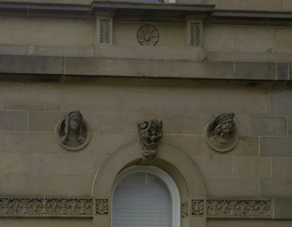
Figure 8 – The exterior carvings
Grid it sideways
We’d never had to consider gridding something that was vertical before, but if using the approach described above, that was what was required in order to capture the heads’ detail. It’s actually reasonably easy to hack – you just need to rotate your data, grid it, then rotate it back (I suspect there may be even easier ways to do it). Doing this allowed us to generate a multipatch, shown on the right in the screenshot below.
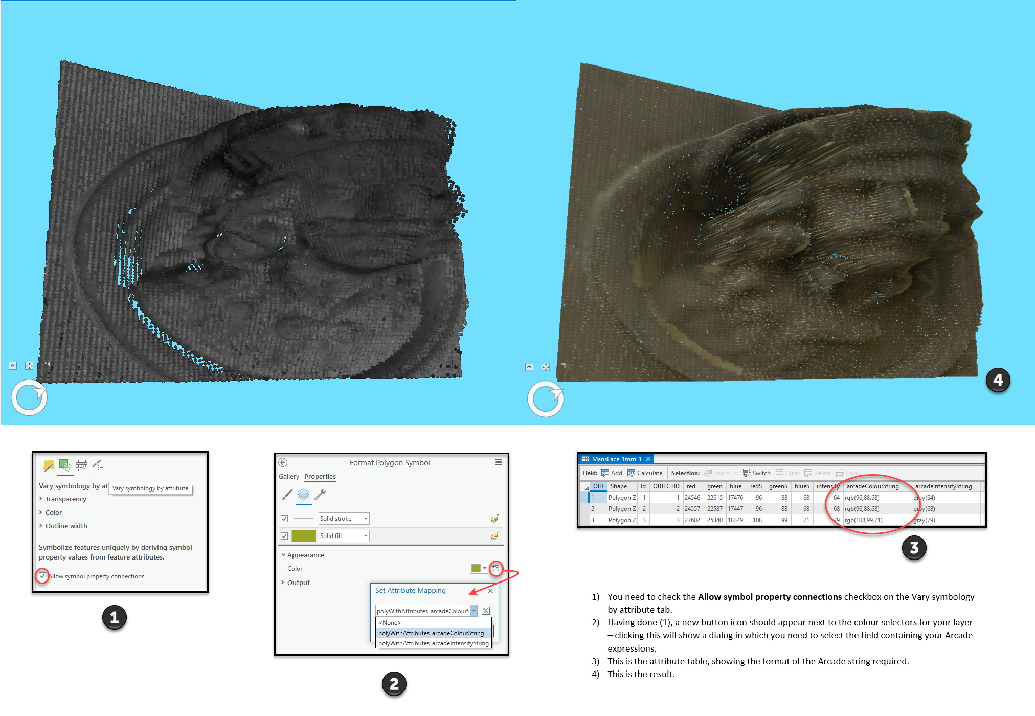
Figure 9 – Converting a vertical point cloud (left) to a multipatch (right)
Styling using Arcade
We incorporated some logic to also interpolate the colour information from the point cloud and add this as attributes, allowing us to use Arcade expressions to style the individual patches by their original colour (attribute-driven symbology)– the screenshot above illustrates the results of this, and provides some guidance as to how to access this functionality: if you click the image you should see a bigger version.
Is that of any use?
There are quite a few issues with that result, but I’d say it meets our requirement of defining a baseline for an object’s state. I think there are better ways of doing it, such as creating a model by meshing (I dare say Drone2Map might be able to assist with that, we will have to try it out), but our aim was to do it within the ArcGIS platform, and we’ve achieved that.
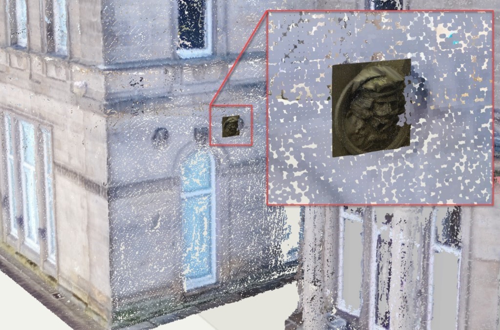
Figure 10 – The 1mm multipatch displayed with the drone point cloud in ArcGIS Online
Creating a 1mm resolution multipatch for the entire office, however, doesn’t seem like a sensible thing to attempt – not least because it would be completely unusable. As many of the surfaces we’re looking to model are relatively featureless, that 1mm resolution dataset would record a lot of nothing. Looking to the future , an image-compression-like-capability for multipatches might improve matters, but for the moment, only capturing high resolution data where we need it and reducing the resolution elsewhere seems a sensible approach – especially if we combine it with those profile lines we were looking at previously.
However, before we get to that, let’s take a brief detour into taking pictures.
Picture it
We were obsessed above with getting lots of detail, and we did – but too much, the things we created were too big. Part of the problem is that they hold a lot of duplicated or deducible information. A picture, in comparison, can provide a comparable amount of information in a much smaller space.
It’s possible to project the point cloud onto planes and then render these to images, using the colour/intensity (or, if you want to side-step the interpolation process described above, the distance between the point and the plane). As you’re defining the plane, you can easily create a multipatch representing it (you can extract the top and bottom Z values from the point cloud), to which you can then apply the image you have rendered, as shown in the screenshot below:
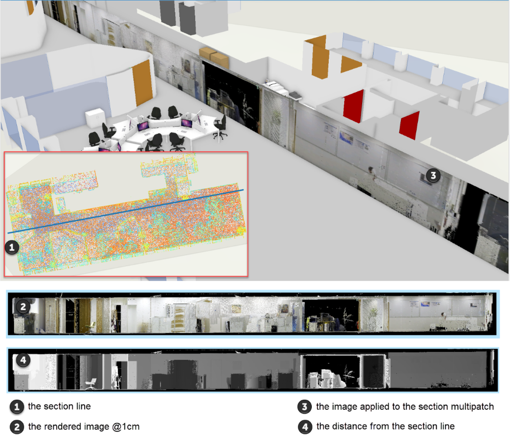
Figure 11 – A rendered section through the point cloud applied to a multipatch
Publishing that textured multipatch (1cm pixels) to ArcGIS Online resulted in an item 315Kb in size, which is tiny. Creating these along the walls, we get a very lightweight ‘photo-realistic’ model. The Slice Multipatch tool is your friend here – you can rotate the basic horizontal and vertical clipping planes it creates to chop your multipatch up and then delete the bits you don’t want, or separate them for viewing purposes.
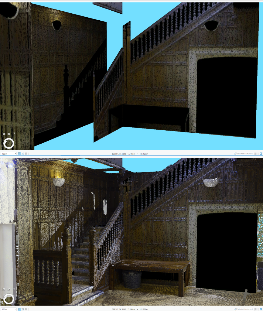
Figure 12 – Top: Simple textured multipatches. Bottom: Same, overlain with the source point cloud
Additionally, where we had pictures on the walls, we clipped these out of the multipatch to create individual digital twin assets.
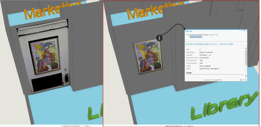
Figure 13 – Extracting features from a multipatch (left) to create digital twin objects (right)
Profile it
Back at the start, we’d looked at manually creating profiles through the point cloud, which we were going to somehow join together to make multipatches. We revisited the idea, but this time we automated the profile extraction and then worked out how to horizontally extrude these profiles along polylines into multipatches. This allowed us to model quite complex shapes, such as the ceiling cornicing, or small features like balustrades and balusters, or the external elevations. It also allowed us to capture the shapes of walls for our basic floorplans. Moving on, using the ArcGIS Pro SDK, we can integrate the ‘pictures’ we took earlier as textures, to create enhanced multipatches showing some of the surface relief.

Figure 14 – integrating a photo section with an extruded profile (profile in red on right)
Extending this approach to allow the use of multiple profiles to define panels is one of the next things on our list for this project – this would, for example, allow us to capture the wood panelling on the staircase accurately.
We hope you’ve found something of interest in this set of blogs; we’ll hopefully be back with some more later in the year, showing how you can integrate IoT sensors into your Digital Twin to gain real–time insights into your environments, and also looking at iPad/iPhone LiDAR scanner data, which seems likely to trigger a boom in DIY Digital Twins.
In the meantime, if you’re interested in discussing how you might create your own Digital Twin in the ArcGIS platform, please do get in touch with us.
Posted by Ross Smail, Head of Innovation.


