In this blog we look at ways in which you can assign depth values to geological features and combine the results of your qualitative and quantitative analysis to generate models of the subsurface.
See our previous blog to learn about the importance of understanding the provenance and resolution of your gravity and magnetic data and also how careful processing and generation of key derivatives can help you quickly build a qualitative understanding of the structural framework of any area.
Magnetic Depth to Basement (D2B) Methods
As discussed in Part 1 of the blog series, a key assumption made when analysing magnetic data is that the sedimentary section is non-magnetic and that the observed magnetic response comes from the top or from within crystalline basement. The presence of intra-sedimentary magnetic sources, such as volcanics, can add complexity and uncertainty to our interpretation but the assumption holds for the majority of cases. This means that when we apply quantitative depth analysis to magnetic data we can be reasonably sure of what target we are assigning depths to. Since the observed gravity response is generated from a multitude of discrete density contrasts within the subsurface, depth analysis of the gravity data is prone to error and is harder to interpret. Therefore, it is not typically employed if good quality magnetic data are available.
Magnetic depth estimation techniques have evolved over the years. In the past, depth estimates were individually generated by hand from profile data by analysing the width and amplitude of magnetic anomalies. Today, there are several semi-automatic techniques that can rapidly return depth estimates from a grid of magnetic data, including;
– Source Parameter Imaging (SPI) Method
The amplitudes at local maxima in the local wavenumber grid are related to the depths to simple magnetic sources (Thurston & Smith, 1997). Phillips et al. (2007) calculated the local wavenumber from the analytic signal and directional derivatives of the RTP and the first vertical derivative of the RTP.
The maxima in the local wavenumber grid can be identified using the ridge tracking algorithm of Hansen and de Ridder (2006). Depth estimates for each maxima can then be produced based upon an assumed source geometry.
The SPI method tends to produce relatively high-resolution results but can be susceptible to noise in the magnetic grid.
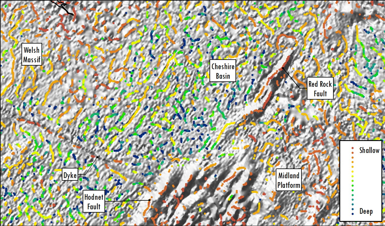
SPI depths, English Midlands. Backdrop is grey-shaded 1st vertical derivative of RTP aeromagnetic data (BGS).
– Tilt Depth Method
Salem et al. (2008) have shown that the zero contour of the Tilt angle locates the edges of vertical magnetic contacts and that the half-distance between the +/-45 degree contours provides an estimate of source depth.
The depths are most reliable where the +/-45 degree contour corridor is linear with consistent width. Depths are less reliable where the corridor is irregular, suggesting complex sources or interference between neighbouring anomalies.
The Tilt method tends to produce lower resolution results than the SPI method but is less susceptible to noise. As such it is particularly useful at delineating the flanks of basins
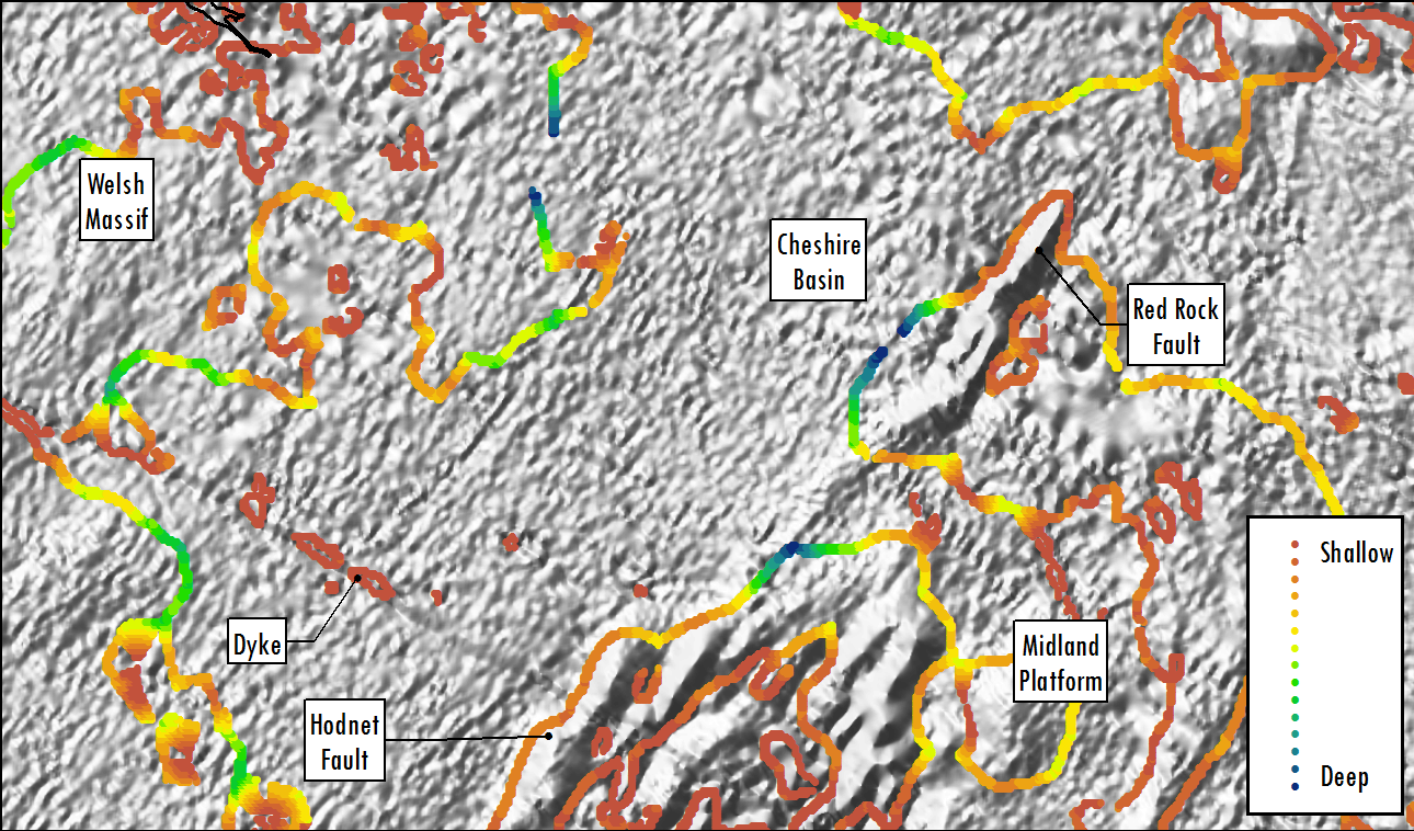
Tilt depths, English Midlands. Backdrop is grey-shaded 1st vertical derivative of RTP aeromagnetic data (BGS).
– 2D Forward Modelling
2D forward modelling allows the user to compare the gravity and magnetic response of a hypothetical geological cross section against observed data. Due to the non-uniqueness of gravity and magnetic interpretation, there will be a large number of geological models which could produce gravity and magnetic anomalies that agree adequately with the observed anomalies.
The key to reducing the number of these alternative models is to apply control in the form of seismic interpretation, well tops, density and susceptibility values derived from logging and sampling, outcrop information and magnetic depth estimates.
A good understanding of the regional geology of the study area can also help eliminate unlikely geological interpretations. By going through the 2D modelling process, the interpreter can shed light on unresolved issues such as:
- How deep is the basement?
- Is the seismic interpretation/depth conversion consistent with the gravity and magnetic data?
- What is the possible make-up of anomalous seismic features: Igneous? Salt? Carbonate? Clastic?
- What type of crust is present: Continental? Transitional? Oceanic?
- How thick is the crust?
- Is the qualitative structural interpretation consistent with the model? Do faults have to be added or removed, moved laterally or the structural style altered?
- Which alternative geological models also fit the observed data?
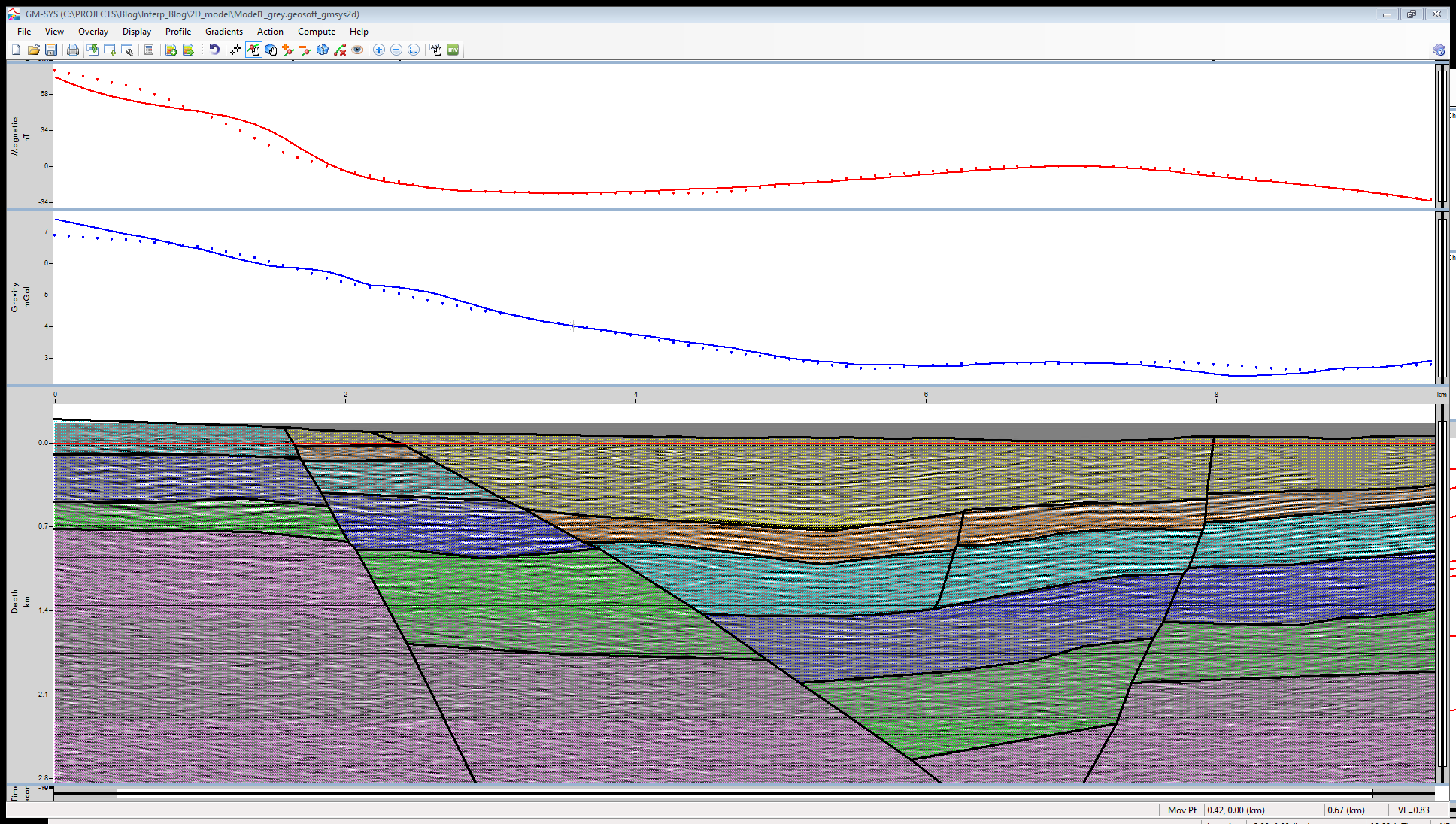
2D gravity and magnetic model along seismic line SAX-85-06, Midland Valley Basin, Scotland (Public domain seismic image courtesy of UK Onshore Geophysical Library). The upper part of the figure shows the observed magnetic data as red dots and the magnetic response of the model as a red line, the middle part of the figure shows the observed gravity data as blue dots and the gravity response of the model as a blue line. The lower part of the figure shows the geological model in depth with the seismic data as constraint.
– 3D Inversion
A gravity (or pseudogravity) grid can be inverted to yield a grid of the depth variation of a specific horizon. Commonly, this might be the base of a sedimentary basin, base syn-rift or some other significant horizon that corresponds with a significant density (or pseudodensity) contrast.
Gravity inversions can often be refined by stripping away the gravity effects of known, seismically defined layers so that the residual anomalies can be more reliably related to variations in the target horizon.
The inversion can be constrained by including reliable depth information from seismic, 2D modelling results, well and outcrop datasets for our target horizon. The most common type of inversion uses a grid of gravity but it is also possible to use the same inversion technique for magnetic data as long as the magnetic grid is transformed into a pseudogravity grid.
A pseudogravity grid is a monopolar transformation of an RTP magnetic grid, which is dipolar, thus showing the gravity grid that would be observed if density were proportional to magnetic susceptibility.
The output depth grid from a 3D inversion will be smooth; similar to the input gravity/pseudogravity grid.
As a further step, it is possible to produce a faulted depth grid similar to those produced from a network of seismic lines. However, this involves utilising the qualitative structural interpretation and thus can be susceptible to interpreter bias.
– Summary
By combining the results of qualitative and quantitative gravity and magnetic data interpretations with supporting geophysical and geological control data (where available) you can generate robust models of the subsurface which can help to reduce exploration uncertainty, provide regional context to prospect-scale exploration and help delineate your targets quickly and at a fraction of the cost of new seismic data acquisition.
Keep an eye out for future Getech blogs and webinars where we will highlight how innovative modelling of potential fields data can improve your understanding of the local thermal regime for maturity modelling and geothermal exploration.
Posted by Matthew Stewart, Senior Geophysicist, Getech.

