As with many geophysical interpretation methods, the analysis of gravity and magnetic data has two distinct aspects: qualitative and quantitative. Qualitative aspects include mapping observed features in a geological context, while quantitative aspects include assigning depth values to anomalous features to generate models of the subsurface. In the first part of this blog series, we’ll discuss qualitative interpretation.
Before we do so, however, it’s essential to understand the various gravity and magnetic fields, what they represent and how we can apply advanced processing methods to highlight detail contained within.
Gravity Data
Typically, gravity data are processed and displayed as either free-air, Bouguer or isostatic anomalies.
- Free-air gravity data have been processed to adjust the data measurements to a common datum (normally sea level).
- Bouguer gravity data goes one step further by correcting for the gravity effect of the mass that lies between the observation height and free-air datum. This correction removes the bulk of the topographic or bathymetric effects that are present in the free-air anomaly, and thus provides a clearer picture of subsurface geology.
- Isostatic gravity data have been further corrected to try and remove the effects of Moho depth variations. The aim of this correction is to restrict the observed gravity anomalies to those that originate from sources within the sedimentary section and crust simplifying and focusing the interpretation.
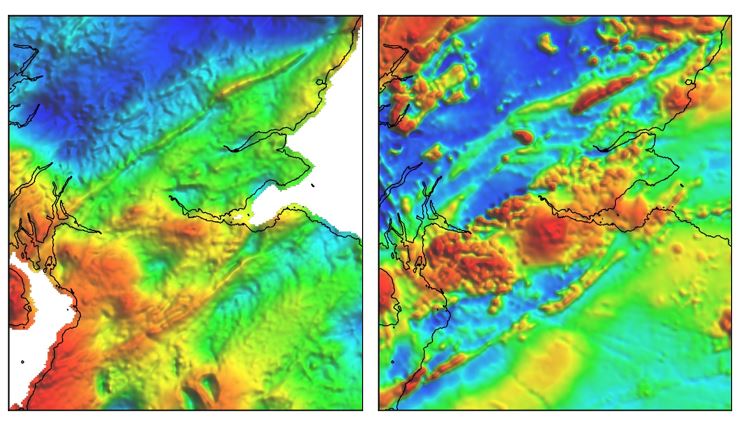
Figure 1: Bouguer gravity (left) and RTP magnetic (right) grids for central Scotland (data from BGS).
Magnetic Data
Magnetic data are theoretically more complex to interpret than gravity data. This is due to two main factors:
- The magnetic field is dipolar, that is, it has two opposite poles (unlike the simpler gravity field, which is monopolar).
- The magnetic response of a given body changes according to location due to the variability of the geomagnetic field over the Earth’s surface.
The second factor can be accounted for by performing a reduction to pole (RTP) transformation, which produces symmetric anomalies that are centred over the causative body. In practice, magnetic data are often easier to interpret as commonly the only magnetic source in the sub-surface is crystalline basement. In contrast, the gravity field is generated by density contrasts located throughout the entire geological section.
Since the bulk of the observed magnetic response usually originates from crystalline basement, it is often best to begin the qualitative interpretation by looking at magnetic data first rather than gravity data. After interpreting the magnetic data we can then seek greater consistency with the longer-wavelength gravity features. Any remaining gravity anomalies (for long or short wavelengths) may thus be linked to, broad, narrow, or shallow sources.
Derivatives and Lineament Mapping
To extract structural detail from gravity and magnetic data, it is often helpful to refine the data using derivatives or filtering. A derivative that is commonly used to highlight structural trends and fault locations is the total horizontal derivative (THD).
This derivative produces maxima where the gravity or magnetic gradients are strongest, highlighting the locations of major density or susceptibility contrasts. This can include faults, the edges of bodies or lateral compositional changes. In other words, we can use this derivative to guide us as to where to put the lines on our maps.
A further step is to apply a Tilt derivative to the THD, which acts like a gain control that will help to highlight subtler gradient maxima in gravity and magnetic data.
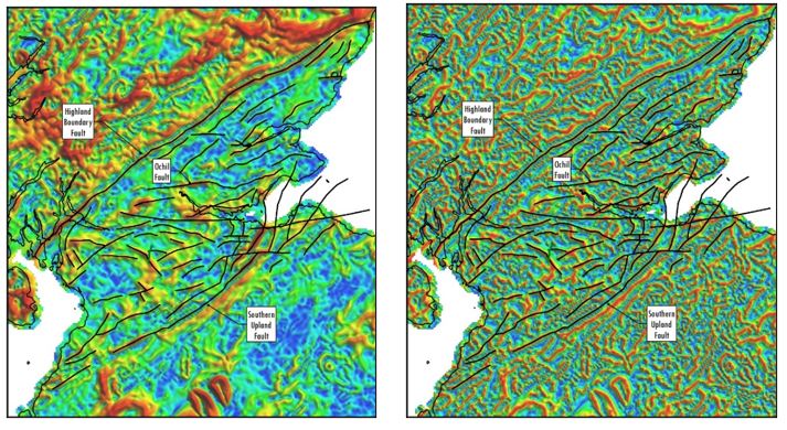
Figure 2: Structural trends of the Midland Valley Basin, Scotland, determined from Bouguer gravity THD (left) and THD Tilt (right).
Geological Context
Once we have identified the locations of the structures within our study area, we can then determine the nature of these structures.
For normal faults, we can determine which side is downthrown by observing the relative magnitude of the gravity or magnetic anomalies on either side of the structure (this may be revised later after quantitative analysis).
For strike-slip faults, we can estimate the amount of lateral movement by correlating older features which have been segmented and offset by the structure.
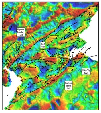
Figure 3: Midland Valley Basin (Scotland) fault interpretation overlain upon 50 km high-pass filtered Bouguer gravity data. Note the offset of the Caledonian Southern Upland Fault inferred to occur on a younger, east-west trending strike-slip fault.
Mapping of Geological Bodies
It is not just faults that we can detect with gravity and magnetic data. Appreciable density or susceptibility contrasts can also indicate the presence of different types of geological bodies (i.e. lateral changes in geology).
For magnetic data, the presence of volcanics can commonly be identified – especially when they are situated within a relatively non-magnetic sedimentary section. In this setting, they become visible through moderate to high-amplitude, short-wavelength anomalies, superimposed upon the lower amplitude, longer wavelength regional magnetic background originating from crystalline basement.
With gravity data it is possible to detect bodies with anomalous densities, for example:
- High-density carbonate reefs juxtaposed against low-density sandstones.
- Low-density salt diapirs piercing higher density sediments.,
- Granitic plutons within higher density crystalline basement.
Granitic plutons can also be identified with the help of magnetic data. Although relatively lowly magnetic, they are often surrounded by a halo of magnetic features related to mineralised zones on their flanks.
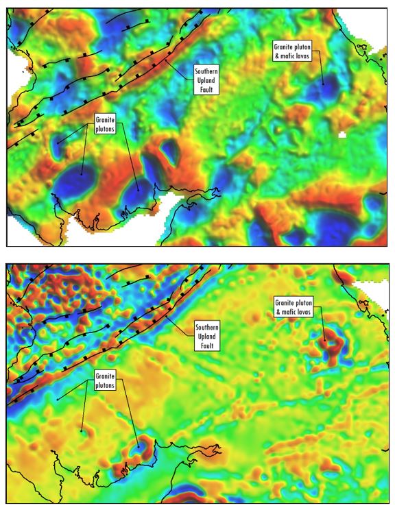
Figure 4: Granitic and volcanic bodies interpreted from gravity (top) and magnetic data (bottom), southern Scotland.
Summary
In this blog, we have introduced how gravity and magnetic data and their key derivatives can be used to quickly build an understanding of the structural framework of any area. This can be an especially powerful tool when integrated with other data such as seismic, to enable the interpreter to develop a geological model away from isolated areas of constraint data.
We have also shown how understanding the gravity and magnetic responses of geological bodies allows us to map the locations and extents of these features even when they are concealed by the overburden.
Look out for part 2 of this blog where we introduce quantitative modelling to further expand our understanding of the sub-surface.
Posted by Matthew Stewart, Senior Geophysicist, Getech.


